<< eutony.net

Aims

The aim of this research was to develop new tools and techniques for analysing data generated using terahertz (THz) pulsed imaging technology. The noise present in terahertz images was examined in detail, joint time-frequency techniques were applied to THz data, and clustering algorithms in time, frequency, and time-frequency based were used to segment THz images into their constituent regions.

This webpage is, of course, only a brief summary of the research and results carried out for this doctorate. Interested readers are referred to the thesis and my other publications for more details.

Background

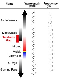
Electromagnetic radiation in the terahertz band, broadly 300 GHz to 10 THz, was first isolated in 1897 but remained largely unexplored in the years following. Falling on the boundary between microwave and infrared, this so-called “terahertz gap” resulted from the failure of optical techniques to operate below a few hundred terahertz, and likewise the failure of electronic/radio methods to operate above a few hundred gigahertz.

Aside from the “because it's there” line of reasoning, the terahertz band is interesting because:

• The universe is naturally bathed in terahertz radiation.
• The radiation is non-ionizing.
• Terahertz radiation is highly sensitive to the presence of polar substances, such as water and thus hydration state.
• ‘Dry’ non-polar substances, such as plastics, fibres, and so on, are almost transparent to terahertz radiation.
• The wavelength is shorter than for microwave wavelengths, with the associated improvement in spatial resolution, while still being long enough to experience less of the Rayleigh scattering experienced by infrared.
• Light weight molecules have strong emission or absorption lines in this region for rotational and vibrational excitations.

Recent advances in laser and electro-optical technologies have enabled bright terahertz radiation to be coherently generated and detected, making this band accessible.

Terahertz Imaging

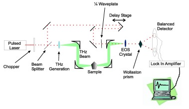
In terahertz pulsed imaging, pulses of terahertz radiation are generated using either non-linear optics or a dipole antenna, steered to interact with a sample, and are subsequently detected in the time domain using similar techniques to the generation. These pulses are recorded via the selective amplification of a lock-in amplifier. The terahertz imager may be set up in either transmission or reflection modality, where the detector is either the opposite side of the sample to the transmitter (transmission mode) or is the same side of the sample as the transmitter, being positioned in such as way as to capture reflections from the sample (reflection mode). The figure above shows a schematic of a terahertz pulsed imaging system in transmission mode.

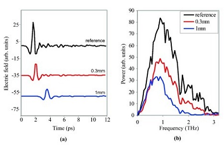
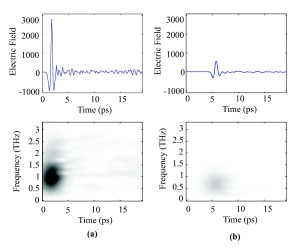
The coherent generation and detection of the THz electric field results in a time-series waveform, which can be transformed into the frequency domain by using the Fourier transform. The figure to the right shows examples of terahertz pulses in (a) time domain, and (b) magnitude of Fourier coefficients. The pulses are very well localised in time, and have a broadband frequency content. Notice that in the time domain the pulses are translated, attenuated, and dilated by vary amounts depending on the thickness of material. The power spectrum shows the pulse frequency content is centred around 1 THz, and that the higher frequency content is attenuated more by nylon than the lower frequencies. This is also suggested in the time domain --- the pulse through 1 mm is a lot smoother, i.e. devoid of high frequency content.

Noise in Pulsed Terahertz Systems

Undesired data and the corruption of signals, or ‘noise’, are issues that affect all ‘real world’ signals, and all signal processing applications must take it into account. The main theoretical sources of pulse noise in terahertz imaging are Johnson noise and shot noise, both of which may be modelled as wide sense stationary Gaussian processes, however we empirically found that the noise present in terahertz signals may be modelled using distributions from the stable family but not using either a single or multiple Gaussian model.

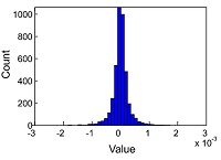
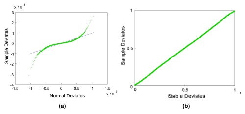
The noise in a terahertz data-set for a given sample was estimated by taking the differences in the time-domain between each terahertz pulse that had passed through that sample and the mean of all those pulses. An example histogram of this noise distribution is shown in the figure to the left. This histogram shows a ‘heavy-tailed’ distribution, i.e. one that has longer tails than a normal distribution, as is shown by a normal probability plot of the data, as seen in Figure (a) below. The green crosses are the data from the distribution, and the straight blue line is the hypothetical normal distribution - the data clearly deviate from the distribution at the ends. Statistical tests show that we cannot have confidence that a normal distribution models this data.
In contrast Figure(b) below shows the stable probability plot, where a stable distribution has been used to model the noise, and here statistically we can be confident the model fits - and the figure shows an almost perfect fit of the model to the data.

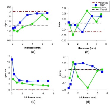
Distributions from the stable family are described in terms of four parameters - α, β, δ, and γ, which are the index of stability, skewness, scale and location respectively. We found a suggestion that both α and γ - which are describing the noise distribution - are dependent on the depth and type of material being imaged. The figure to the left shows how these parameters vary with sample and sample thickness. Each subfigure shows a different parameter, with (a), (b), (c), and (d) showing α, β, δ, and γ respectively. The blue and green lines show the parameters plotted against thickness for resin and nylon respectively. The dashed red line shows the parameter values obtained when all the THz radiation is blocked, and the black dashed line shows the parameter values when the radiation passes through free-air. In both these cases, sample thickness has no meaning.

Extreme denoising was applied using Donohoe's wavelet shrinkage algorithm in an exploration of possible compression techniques, and we found that the refractive index and absorption coefficient values remained essentially unchanged even when only 20% of the original wavelet coefficients were stored.

Terahertz Imaging: Using Optical Parameters as a Contrast Mechanism

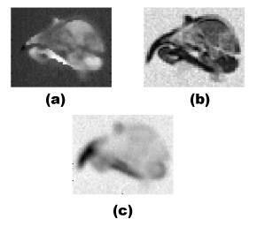
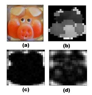
Terahertz data has a high dimensionality - sometimes 512 time samples are ‘behind’ every pixel of a terahertz image. Some sort of processing needs to be carried out before pictures can be created. Typically parametric images are formed, using time or frequency based observations such as peak to peak time difference, or relative transmission. The two figures below show examples of such images. The left figure shows a cross section of a bird's skull, with images formed from (a) peak to peak time difference, and the relative transmission at (b) 1 THz and (c) 0.41 THz. The right figure is of the head of a marzipan pig, with images formed from (a) an optical photograph, (b) peak to peak time difference, and relative transmission at (c) 1 THz and (d) 0.31 THz.

The images above rely on the optical parameters of the sample in order to create a contrast between pixels of the image, and we developed this technique further using a short term Fourier transform (STFT), and a wide-band cross ambiguity function. The figure to the right shows the time domain and corresponding spectrogram for a terahertz pulse through free air (a) and through 2mm of nylon (b). The grey level represents the mutually normalised magnitude of the coefficient, with black indicating 1 and white indicating 0. Notice that the retardation of the pulse by the nylon is visible in the STFT spectrogram, as the larger coefficients (denoted by darker grey level) are further to the right than the reference pulse. The attenuation is also visible, as the coefficients are all smaller (lighter grey levels). Finally pulse broadening can be seen, as the widest part of the nylon pulse's STFT coefficients is wider than those of the reference pulse's STFT.

We show that the STFT with a normal window is a promising tool for the calculation of optical parameters, and may be especially of value in reflection imaging, where a joint time/frequency distribution enables frequency content to be examined at a specific time. The cross-ambiguity function showed itself to be capable of distinguishing between nylon and resin based on the optical parameters, however the results were not entirely consistent with traditional analyses, raising some questions over its reliability.

Approaches to Segmentation of Terahertz Pulsed Imaging Data

Terahertz pulsed imaging delivers data of a high dimensionality, which raises the possibility of clustering techniques to segment terahertz images into their constituent regions. Groups of pixels which are ‘similar’ in some way are clustered together, and an image may then be formed by the assignment of different colours or greyscale levels to these groups. These images may then either be used as an end in themselves, or alternatively could be used as a first step that highlights potential areas of interest for further analysis.

For this analysis, k-means clustering was applied to terahertz data, based on both high dimensional vectors formed from temporal, spectral, and combined domains, and on low dimensional vectors formed by extracting specific features such as absorption at a given frequency. The terahertz data used was synthetic transmission data of a slice of tooth, real transmission data of a slice of tooth, and real reflection data of three specially prepared phantoms made of painted stickers on TPX ¹. Highlights of these results follow.

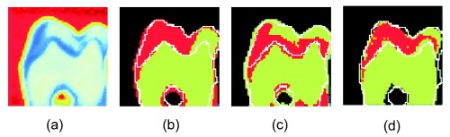
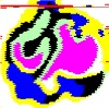
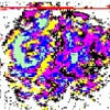
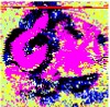
The figure below shows the results of the segmentation of the real slice of tooth, using k-means clustering on (b) the time series, (c) the FFT coefficients, and (d) a 3D feature vector. (a) shows a false colour relative amplitude picture for comparison. The white lines show the boundaries between the regions of the tooth extracted from the hand-segmented radiograph. Between 77% and 87% of pixels were correctly classified in this way (depending on clustering metric).

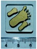
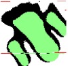
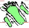
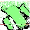
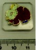
This process was repeated with the manufactured phantoms. The figure below shows a photograph (a) and hand-segmented ground truth (b) for the ‘foot’ phantom (top) and ‘rabbit’ phantom (bottom). Results for clustering are show in the figures (c), (d), and (e), corresponding to the time series, FFT coefficients, and a 3D feature vector as before. In this case 60 - 80% of the foot pixels were classified correctly, and 35-50% of the rabbit pixels were.

This exploration was highly speculative, but was nonetheless encouraging for the tooth transmission images. The phantoms faired less well, but these were designed to be imaged in transmission mode, while unfortunately time and machine constraints forced us to image them in reflection mode.

This research degree was jointly supervised by the School of Computing (within the vision group), and by Medical Physics (at the Centre of Medical Imaging Research, or CoMIR). Links to these research groups may be found at the bottom of the page. My supervisors were:

• Prof Roger Boyle, School of Computing.
• Dr Elizabeth Berry, Academic Unit of Medical Physics.
• Dr Anthony Fitzgerald, Academic Unit of Medical Physics - played a supervisory role in the early and middle stages of my PhD

My research was funded by an award from the Engineering and Physical Sciences Research Council (EPSRC). For more information, visit their website (www.epsrc.ac.uk).

<< eutony.net

¹TPX, or or poly 4 methyl pentene-1, is a low loss polymer that is almost transparent at terahertz frequencies.